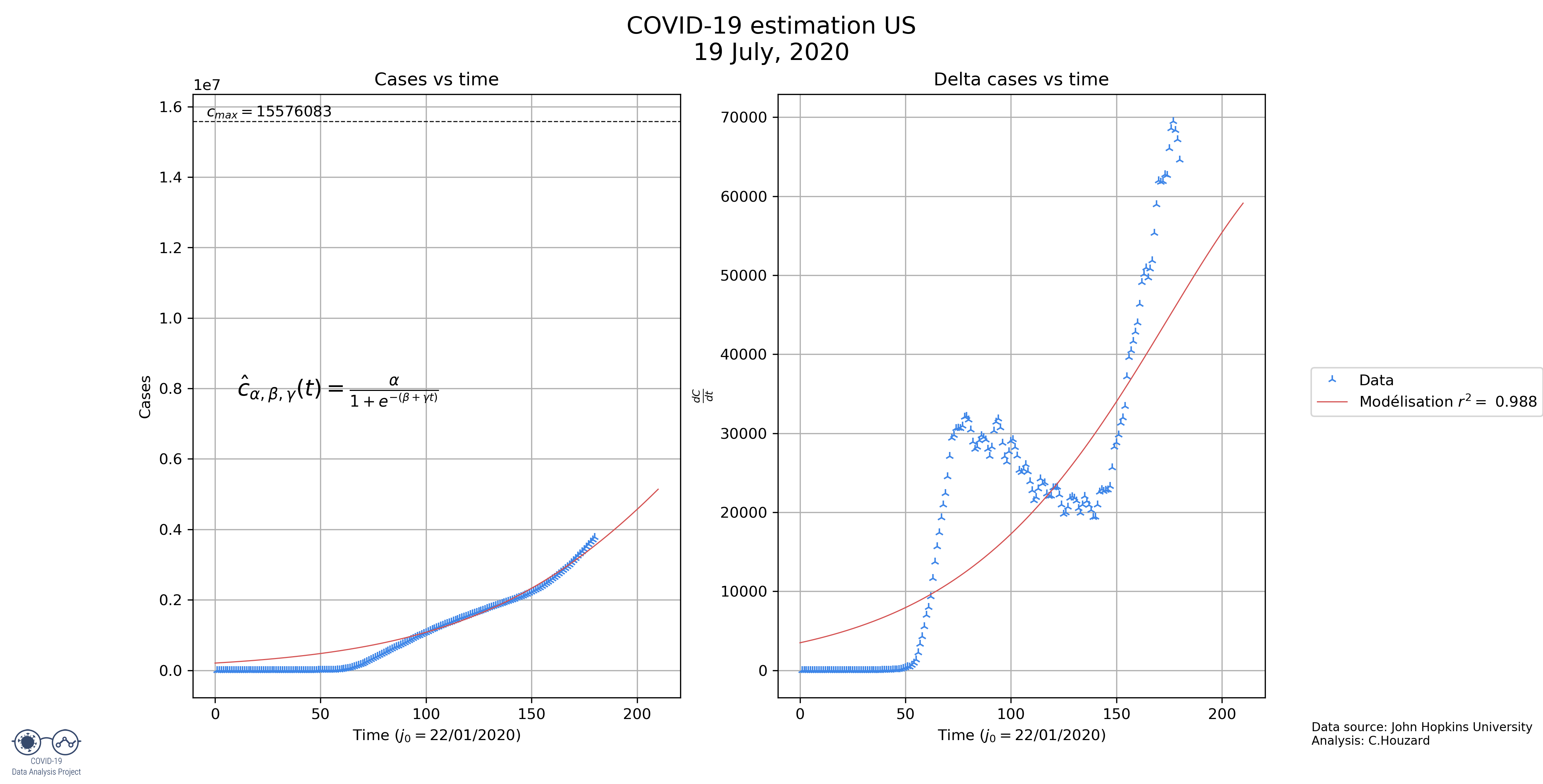
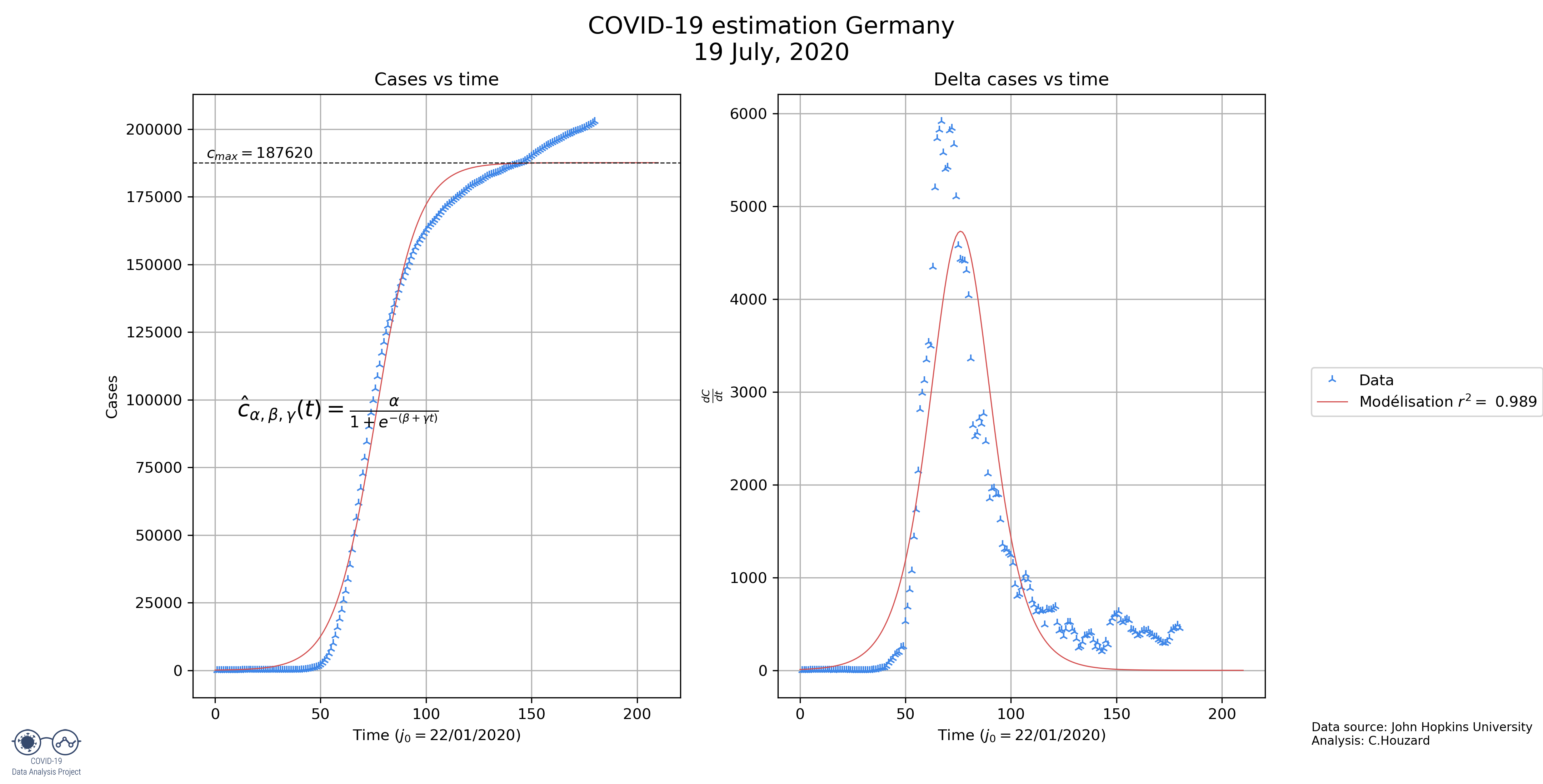
Prediction of the epidemic final size – COVID-19 Data Analysis Project

This article was originally published on Apr, 28. The graphs and values are updated regularly at the end of this article.

Abstract: The purpose of this article is to predict the final size of the COVID-19 epidemic based on a logistic regression model by fitting the data of France, the US, Italy and Spain.

In this article, it will be tried to predict the final size of the COVID-19 epidemic per country based on a logistic regression.

It is divided in 3 parts:

Logistic regression: the properties of this function will be explored
Fitting of the model: it will be described how the best fit was chosen
Results: the model will be applied to 4 countries: France, the US, Italy and Spain
Conclusion
Updated prediction

The codes that were used for these graphs are available on this GitHub repository. The code used for the visualisation of the RMSE (§2.1) is 32 – Visualisation of RMSE.py. The one used for the prediction is 31 – Modélisation v2.0.py (§2.2 and §3).

1. Logistic regression

1.1. Models to predict an epidemic

An epidemic can be described by many models, more or less complex. The most usual models are the compartmental one. They are called this way because they divide a population into categories. For example, the most basic compartmental model is the SIR: Suspected (i.e. not yet infected), Infectious and Recovered. It can give interesting insight on an epidemic like the number of people one can infect on average.

On this model, the infectious curve is essentially a logistic regression if the constants of the model don’t change. Hence, for simplicity, we will consider here that the number of cases follows a logistic regression. Such an application $c$ can be expressed as a function of time with 3 parameters: $\alpha, \beta, \gamma$

$\displaystyle c=\frac{\alpha}{1+e^{-(\beta + \gamma t)}}$

1.2. Properties of a logistic regression

The function $c$ defined above is clearly $C^\infty$ , hence, we can determine the first few derivates.

From these, nice properties can be found. They are summed up in on this graph:

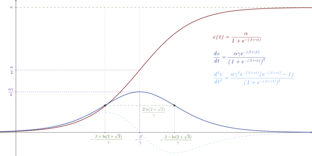
Fig. 1.1 – Representation of a logistic regression, its first and second derivate

1.2.1. Maximum of the function

Finding the maximum of this function presents an obvious interest in our problem: it is the final estimated size of the epidemic. For a logistic regression, we have:

$\displaystyle \lim_{t\to\infty} c(t) = \alpha$

1.2.2. Inflexion point

The function clearly presents an inflexion point. Let’s call it $P_I$ . We have:

$P_I=(-\frac{\beta}{\gamma}, \frac{\alpha}{2})$

By definition, the inflexion on the function $c$ is also a maximum (or a minimum) of the derivate $\frac{dc}{dt}$ . Let’s call this maximum $P_{I'}$ . We also have:

$P_{I'}=(-\frac{\beta}{\gamma}, \frac{\alpha \gamma}{4})$

1.2.3. Growth speed

Let’s focus on the interval $\left]-\infty, -\frac{\beta}{\gamma} \right]$ .

By looking at the 2nd derivate $\frac{d^2c}{dt^2}$ , we can see that the function increases more and more rapidly up until a point we shall name $t_1$ . The 2nd derivate then decreases. Before that point, the growth is essentially exponential.

By solving $\frac{d^3c}{dt^3} (t_1)=0$ , we get :

$\displaystyle t_1=-\frac{\beta+\ln(2+\sqrt{3})}{\gamma}$

Similarly, on the interval $\left[-\frac{\beta}{\gamma}, \infty \right[$ , the growth decreases slower and slower, until $t_2$ , when it starts decreasing faster. The solution to equation $\frac{d^3c}{dt^3} (t_2)=0$ on this interval gives us:

$\displaystyle t_2=-\frac{\beta-\ln(2+\sqrt{3})}{\gamma}$

The difference between these 2 points $t_2$ and $t_1$ gives us a first characteristic time $\tau$ . It expresses the time it takes to go from an exponential increase to an exponential decrease:

$\displaystyle \boxed{\tau=-\frac{-2\ln(2+\sqrt{3})}{\gamma}}$

1.2.4. Total duration of the epidemic

It can be interesting to quantify the time $t_x$ at which the function has reached the proportion $x$ of its final value i.e. at which it reaches the value $x \alpha$ .

By solving a simple equation, $c(t_x)=x\alpha$ , we find that:

$\displaystyle t_x=-\frac{1}{\gamma} \ln \left( \frac{x}{1-x} \right) - \frac{\beta}{\gamma}$

Now we can imagine a new characteristic time that would be defined as the required time to go from the proportion $(1-x)$ to the proportion $x$ . Let’s call it $\Delta t_x$ .

For example, $\Delta t_{99}$ would be the time it took to go from 1% to 99% of the final value $\alpha$ .

It can be expressed as a function of $\gamma$ or $\tau$ :

$\displaystyle \boxed{t_x=\frac{1}{\gamma} \ln \frac{x^2}{(1-x)^2}}$

These values will be used to characterise the epidemic afterwards.

2. Fitting of the model

Now, let’s see how we can fit that logistic function to our data.

For the rest of this paragraph:

Let our data set, the number of cases, be $(c_i)_{1\leq i\leq n}$ . Each $c_i$ is a function of the time $t_i$ where $t_i \in (t_1, ..., t_n)$ .
$(\hat{c_i})_{1\leq i\leq n}=(\hat{c}(t_i))_{1\leq i\leq n}$ is the predicted number of cases at time $t_i$ (where $t_i \in (t_1, ..., t_n)$ ).

2.1. Cost function

2.1.1 What cost function to use?

To fit the model to the data, we need a cost function i.e. a function that expresses how far the model is from the data. This function inputs are the parameters $\alpha, \beta, \gamma$ and the output is a number representing the error. By minimising this cost function, we get the parameters $\alpha, \beta, \gamma$ that fit best the data.

To find the minimum of this function, a gradient decent algorithm is used. This type of algorithm works by following the steepest decent of gradient of the function i.e. by finding which direction will have the lowest derivate.

A good cost function is convex i.e. if we find a minimum, we can be sure that this local minimum is also global one. For example, in $\mathbb{R}^2$ , the function $x\mapsto x^2$ is convex. There is only one local minimum (for $x=0$ ) and it also is a global minium.

Let’s give a real-life example to explain this notion: Imagine being at the top of the mountain, you need to find the bottom of the valley because of the poor weather condition. Now because of the fog, you can’t see any further than your shoes. To find the valley, you’ll likely follow the path that seems to be the steepest. If the mountain is a simple slope, no problem, you will find your way. Now if there is a lake in the middle, you may end up at the bottom of the lake thinking you are at the bottom. This is exactly the same here, we don’t want our mountain to have a lake in the middle.

.Fig. 2.1 – Representation of the Gradient Descent Algorithm

When fitting a linear model (i.e. if $\hat{c}(t)=at+b$ ) the Root Mean Square Error cost function is used. It can be expressed as:

$\displaystyle RMSE(a, b)= \sqrt{ \frac{1}{n} \sum_{i=1}^{n} (c_i-(at_i+b))^2 }$

Here, no matter the initial value chosen, the gradient descent will find a local minimum that is also a global minium.

However, since the logistic regression function is not convex, this cost function can’t be convex.

But, we can work around that problem, and still use the $RMSE$ function by choosing the initial values $(\alpha_0, \beta_0, \gamma_0)$ with much consideration.

Conclusion: to find the best model that will fit the data, we will find the global minimum of the following function:

$\displaystyle RMSE : \begin{cases} \mathbb{R}^3 \to \mathbb{R} \\ (\alpha, \beta, \gamma) \mapsto \sqrt{ \frac{1}{n} \sum\limits_{i=1}^{n} (c_i-\frac{\alpha}{1+e^{\beta + \gamma t_i}} )^2} \end{cases}$

2.1.2. Finding the right initial values $( \alpha_0, \beta_0, \gamma_0)$

For the next two paragraphs, we will consider the French cases from Jan, 20 to Apr, 27. The data are smoothed by a 5 days rolling average (day-2 to day+2). The optimal function was found to be:

Fig. 2.2 – Optimal prediction for French data set ranging from an, 20 to Apr, 27.
$(\alpha, \beta, \gamma) = (126 676, -10.149, 0.139)$

Let’s justify why this is the best fit.

First, it is a matter of choosing the right initial values $(\alpha_0, \beta_0, \gamma_0)$ .

It was observed that if the initial value $\alpha_0$ is too low, the cost function will be minimized for a set of $(\alpha, \beta, \gamma)$ that clearly doesn’t fit the data as it can be seen bellow. Let’s investigate why.

Fig. 2.3 – Example if $\alpha_0$ is too low
$(\alpha, \beta, \gamma) = (74452, -4, 1.1)$

It was also observed that when the predictions were off because of a too low $\alpha_0$ , the final value of $\gamma$ was around $\gamma=1.1$ , instead of $\gamma=0.1$ when the model fits well.

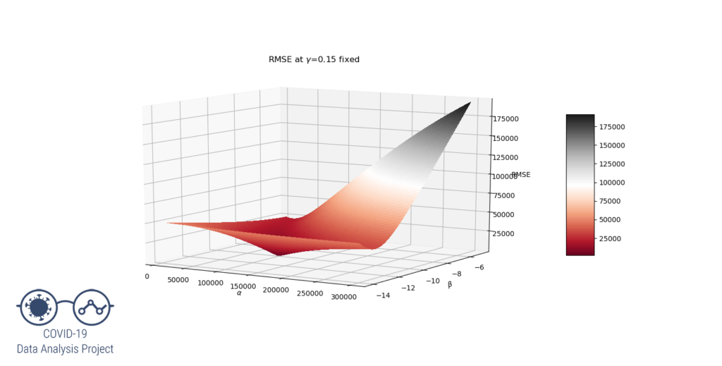
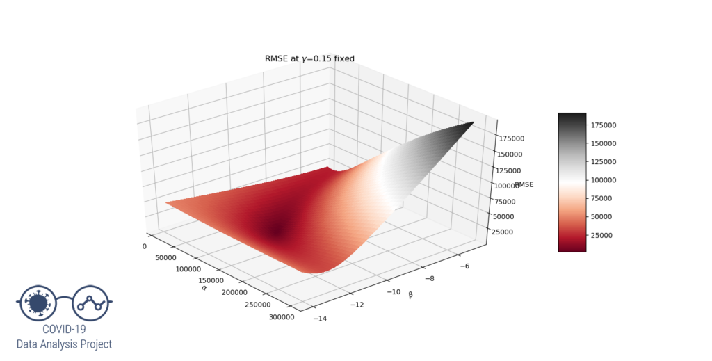
Let’s try to understand why by representing the RMSE function. As this is a 3 variables function and we can’t see 4D graphs (yet…), let’s set the $\gamma$ value at 0.15 and have $(\alpha, \beta)$ vary on a large range. We get the following graph:

Fig 2.4.a – RMSE function for the same data set at $\gamma=0.1$
View 1/2

Fig 2.4.b – RMSE function for the same data set at $\gamma=0.1$
View 2/2

We clearly see that for $\gamma=0.15$ the RMSE function have a local minimum at the desired values of $(\alpha, \beta)\approx(130000,-10)$ that produces a good fit.

Now let’s see what our RMSE function looks like at $\beta =-4$ and $\beta =-8$ .

Fig 2.5.a – Representation of the RMSE at $\beta = -4$

Fig 2.5.b – Representation of the RMSE at $\beta = -8$

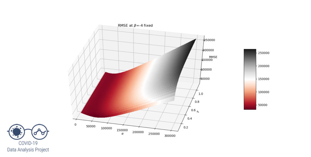
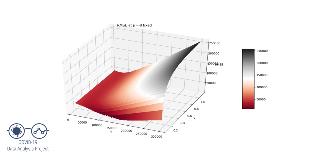
It is clear that around these values of $\beta$ , $\alpha_0$ is too low ; the gradient descent algorithm will get stuck in a set of local minima, we could call it a « valley ».

Also, the higher the beta value, the worse it is. It can be seen that if the beta value is low enough, another local minimum is formed for $\gamma\approx0.1$ and $\alpha\approx150000$ . This is the solution we are looking for.

Conclusion: to avoid ‘falling’ into local minimum, the initial values should be set as:

$\displaystyle (\alpha_0, \beta_0, \gamma_0) = (1.1 c_n, -15, 0.001)$

The code is available here.

2.2. Choosing the best fitting

To find the best match, it is possible to only select a sub set of data $(c_i)_{j\leq i\leq n}$ (with $0\leq j \leq n-30$ ) of the available data i.e. starting at day $t_j$ instead of day $t_0$ . Indeed, at the beginning, the growth was slow and the first $j$ data may not make sense. Also, the parameters of the epidemic growth changed with the confinement. Let’s plot, still for France, the value of $\alpha$ and of $r^2$ as a function of the day at which the date set started $j$ .

It can be seen that the less values are taken (i.e. the higher the $j$ ), the highest the prediction for $\alpha$ is and the lowest the correlation coefficient $r^2$ is.

Fig 2.6 – Evolution of the maximum number of cases predicted and correlation coefficient as a function of the first date of the data set

Now which prediction should be chosen: the one that fits the data the best (i.e. we chose the model that has the maximum $r^2$ , here the sub data set starts on day 30) or the one that is the more pessimistic (i.e. we chose the model that has the maximum $\alpha$ , here the sub data set starts on day 60)?

The model that fits the data the best will be called the $\max (r^2)$ model while the model that is the more pessimistic will be called the $\max(\alpha)$ .

To make the right choice, it was decided, to see how these predictions evolved as time passed. Let’s see them as if the were made on a certain date $t_n$ . This will be the $x$ axis. i.e. we will be plotting as if the algorithm was launched on Apr 06, Apr 07, …, Apr 25.

On the first plot, there will be the prediction for the final number of cases if the chosen model were the most pessimistic (i.e. $\max(\alpha)$ and, on the same plot, what the prediction for the final number of cases would have been if the chosen model were the « rightest » one (i.e. $\max(r_2)$ .

On the right the graphs represent the value of $r^2$ for the two types of selection.

Fig. 2.7. – (*left*) Evolution of the maximum number of cases predicted if the chosen model is the one with the highest $\alpha$ (red) or if the chosen model is the one with the highest $r^2$ , (blue) as a function of when the prediction was made.
Fig 2.7 – (right) Evolution of the correlation factor if the chosen model is the one with the highest $\alpha$ (red) or if the chosen model is the one with the highest $r^2$ (blue), as a function of when the prediction was made.

We can see that, as days go by, the predictions are getting more and more pessimistic. Hence, selecting the curve with the best correlation coefficient wouldn’t be wise. This phenomenon can be explained by looking at the derivate on the graph at the top of §2.2 (the selected model was the one with the highest $\alpha$ value). We can see that the number of new cases daily decreases much slower than the model would predict. It even was stable for about 10 days. This phenomenon will tend to increase the length of the epidemic and so the final $\alpha$ value.

The increase of the number of cases should be as fast as the decrease, but here we see that, on the Figure 2.2, the decrease is slower.

2.3. Summary

This second paragraph can be summed up in 3 points:

The logistic regression model will be fitted using the RMSE cost function

$\displaystyle RMSE(\alpha, \beta, \gamma)= \sqrt{ \frac{1}{n} \sum_{i=1}^{n} (c_i-\hat{c_i})^2 }$

The initial values for the search of the optimal solutions will be

$\displaystyle (\alpha_0, \beta_0, \gamma_0) = (1.1 c_{t_n}, -15, 0.001)$

The algorithm searches the model made with the best sub-set of data $(c_i)_{j\leq i\leq n}$ (with $0\leq j\leq n-30$ ). It selects this best subset by finding the one for which the prediction for $\alpha$ is maximum.

3. Results

The code is available here.

3.1. Predictions

Now that we’ve built a model, let’s apply it to 4 countries: France, the US, Italy and Germany.

We can deduce a few things from these graphs:

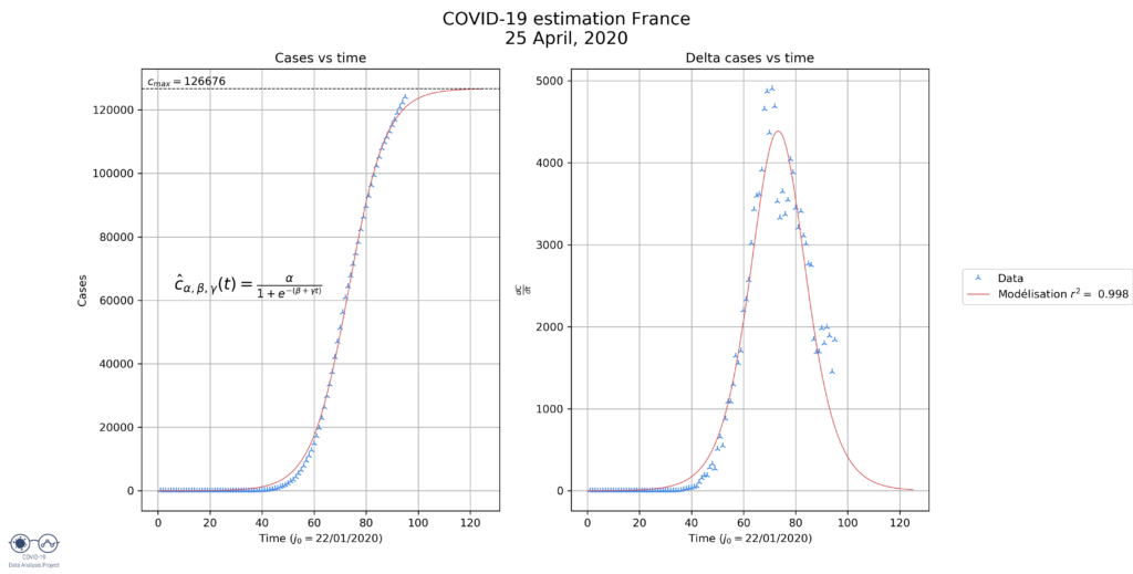
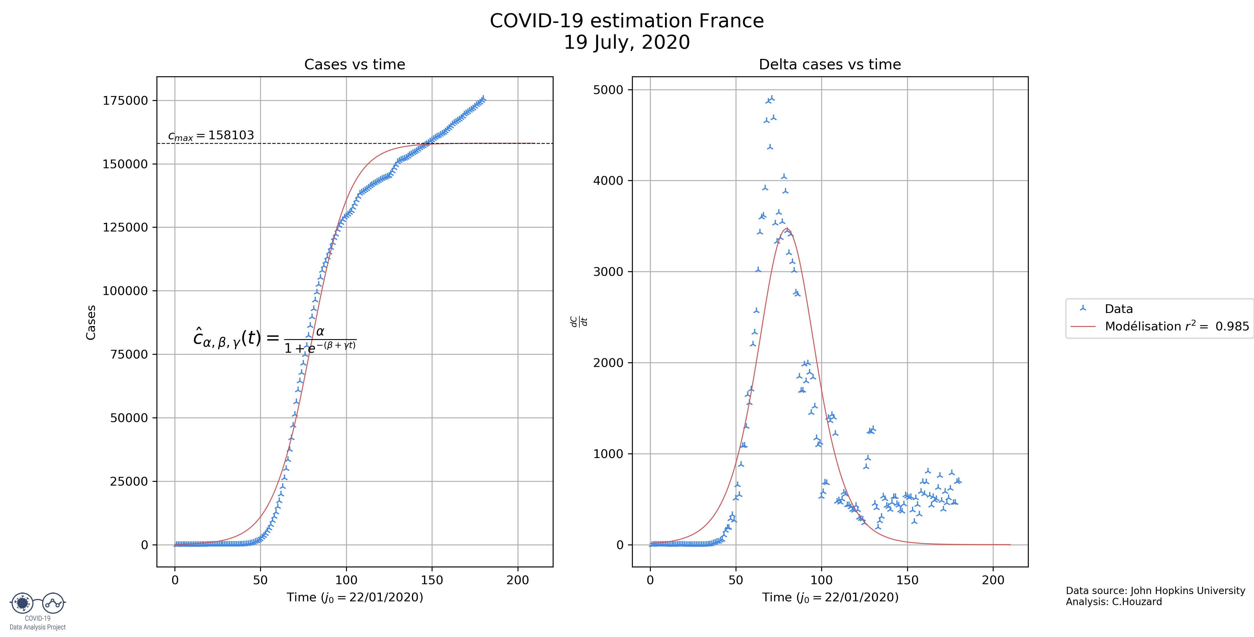
France: the model seems to be underestimating the final size of the epidemic. However, when we look at the derivate, the maximum value was obtained on day 66. On day 66 the total number of cases was around 91 000, which should put the final number of cases around 182 000. This shows partly why the model underestimates the final number of cases (126 000).
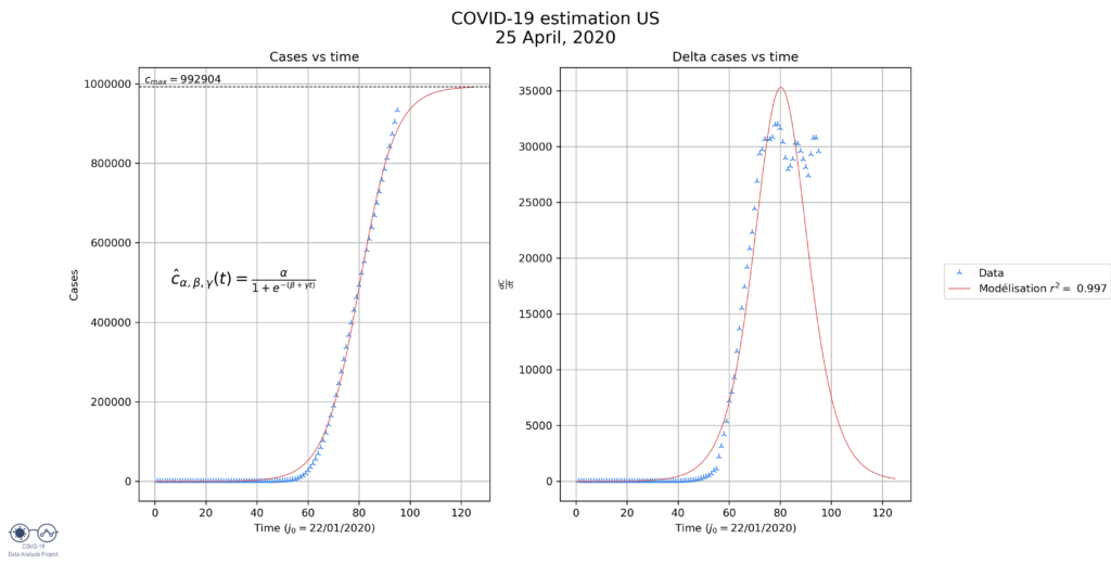
US: Here the model also underestimates the number of cases, indeed, the derivate seems to show us that we are at half of the epidemic, not 94%, as predicted. The model predicts this because the US have been experiencing a constant number of new cases for the past 15 days. The model should readjust when this phase is over.
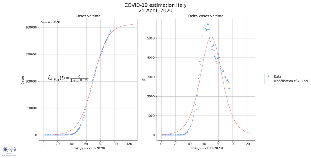
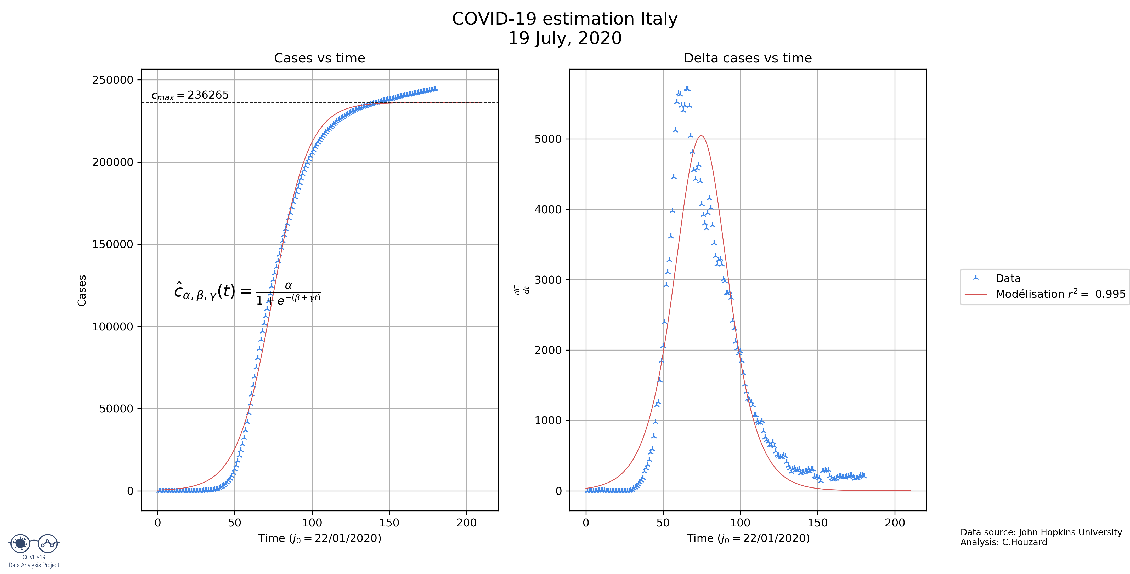
Italy: the model seems to be quite fitting. This makes sense because the decrease of the number of cases in Italy has been quite continuous, more than in France for example.
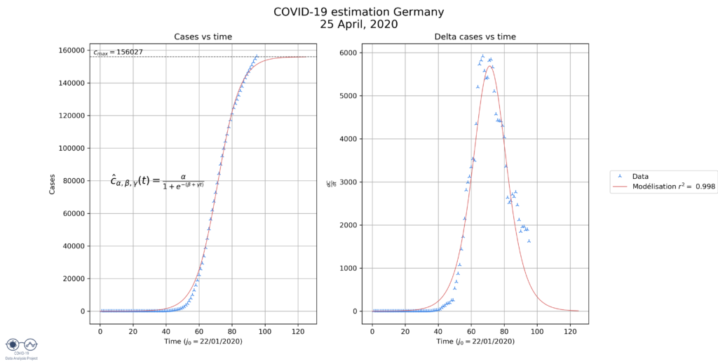
Germany: here the model is clearly underestimating the final size by a lot. That is harder to explain why.

3.2. Comparing the 4 countries

First let’s take a look at the values that are defining the models:

	$\alpha$	$\tau$ (days)	$\Delta t_{99}$ (days)
France	126 676	19.0	132.8
US	992 904	18.5	129.3
Italy	206 281	26.8	187.3
Germany	156 027	18.1	126.0

With these results it can be deduced:

The country with the most cases will be the US, even if the number here is largely underestimated.
Italy will be the country with the longest epidemic, it is supposed to last around 6 months, with them reaching 99% of their cases on May, 16.
The US had a very fast increase and so, we predict a very fast decrease. That remains to be seen.

4. Conclusion

We have seen that the logistic regression function can be used to model the COVID-19 epidemic in various countries. However, this is a very simple model that is far from perfect but can give a good first approximation of what the future will hold.

This model, but also any models, of course, cannot predict what will happen if the context changes e.g. if restrictions are lifted, the number of cases would probably rise sharply.

5. Updated predictions

Below the latest prediction. The algorithm was changed on May, 1. It now prefers to improve the fit on the latest data at the cost of losing in precision with the first values.

First, you’ll find the latest prediction, then you’ll find how these predictions evolve as day pass by.

Reminder: these predictions are built from the situation in the past few weeks. It doesn’t account for the new rules that are applied little by little around the world which could lead to a 2nd wave.

NB: from May, 25 we are experiencing some issues for the German predictions.

Definition of the parameters:

$\alpha$ value: final number of cases
$\tau$ : duration to go from an exponential increase to exponential decrease
$\Delta t_{99}$ : duration to go from 1% of the final number of cases to 99% of the number of cas
Date_99: Date at which 99% of the cases will be achieved
$r^2$ or correlation coefficient: number that evaluates how well the model fits the data, the closer to 1, the better

Values defining the predictions:

	$\alpha$ (number of cases)	$\tau$ (days)	$\Delta t_{99}$ (days)
France	144985	30,53959	213,3501
US	2230283	53,53649	374,0068
Italy	235415	37,85915	264,4847
Germany	178158	30,96605	216,3294

Evolution of the parameters as a function of when the predictions were made:

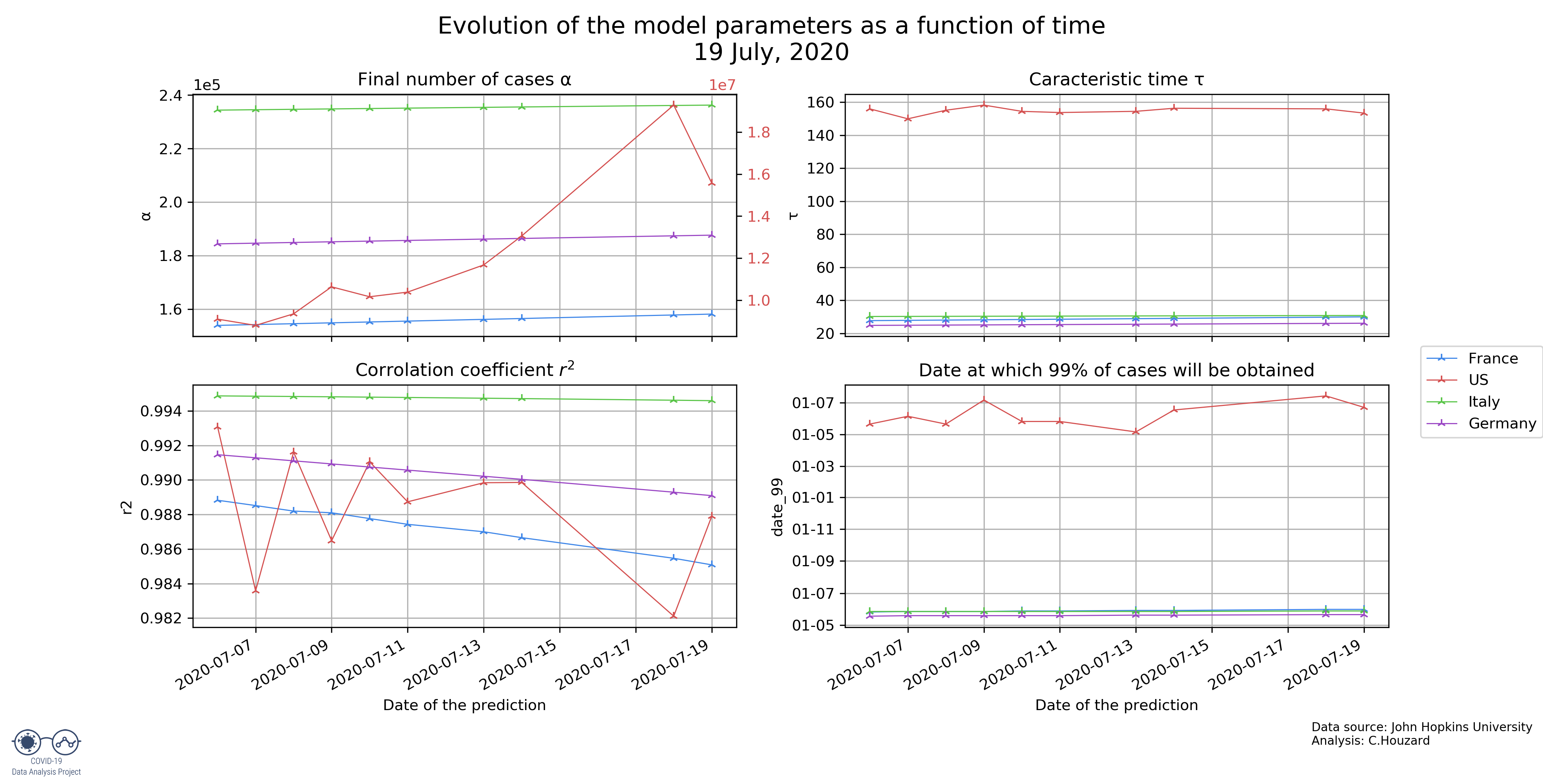
We can see that for France, Germany and Italy the number of cases predicted is getting constant, hence the predictions are more and more precise.